Embedded Python/NumPy in MonetDB
Python is one of the most popular languages in Data Science. It is a flexible scripting language that is easy to use and has a large amount of available statistical libraries. When we’re doing statistical analysis in Python, we naturally need data accessible to us in Python in some way. And what better place to keep data than in a database.
Previously when you wanted to combine MonetDB and Python, you had to use the Python MAPI client. This client suffers from very low transfer speeds because it uses sockets. If you want to execute Python functions on larger data sets this low transfer speed quickly grows out of control.
This is why we are now introducing MonetDB/Python, in which we allow users to create their own Python functions as they would create SQL functions. The embedded python functions can then be used within SQL statements. We show that our new method of making data available to Python analyses is faster than competing solutions.
By using Numpy arrays, which are essentially Python wrappers for C arrays, our Embedded Python implementation can transfer data from MonetDB to Python without unnecessarily copying the data, which leads to extremely fast transfer speeds. In addition, Embedded Python supports mapped operations, which allows you to run python functions in parallel within SQL queries. Combined with the numpy/scipy libraries, which contain very efficient C implementations of numerous statistical/analytical functions, Embedded Python matches the speed of native SQL functions, while offering all the flexibility and ease of use of the Python scripting language. In addition, you can load any of the numerous available Python modules and use them.
Embedded Python works by creating a SQL Function that contains the Python code to be run. A simple function that multiplies the input by two is as follows.
CREATE FUNCTION python_times_two (i INTEGER) RETURNS INTEGER LANGUAGE PYTHON
{
    return i * 2
};
After creating this function, we can use it in a SQL query as follows.
CREATE TABLE integers(i INTEGER);
INSERT INTO integers VALUES (1), (2), (3), (4), (5);
SELECT python_times_two(i) AS result FROM integers;
| result |
|---|
| 2 |
| 4 |
| 6 |
| 8 |
| 10 |
Data Input
Now you might be wondering what exactly “i” is in this function. As we have mentioned previously, we are using Numpy for converting between MonetDB and Python. The exact type of “i” depends on the input; if the input contains a NULL value, “i” will be a MaskedArray, otherwise “i” will be a regular one-dimensional Numpy array. The dtype of the array depends on the type specified in the SQL function. In this example the specified type is “INTEGER”, which corresponds to a dtype of numpy.int32. Below is a table that contains the exact types for every possible input value.
INPUT          DTYPE
BOOLEAN        numpy.int8
TINYINT        numpy.int8
SMALLINT       numpy.int16
INTEGER        numpy.int32
BIGINT         numpy.int64
REAL           numpy.float32
FLOAT          numpy.float64
HUGEINT        numpy.float64
STRING         numpy.object [1]
Creating Tables using Python Data
We can also use the embedded python to create tables or insert data into existing tables. Consider the following function.
CREATE FUNCTION python_table()
RETURNS TABLE (name STRING, country STRING, age INTEGER)
LANGUAGE PYTHON
{
    result = dict()
    result['name'] = ['Henk' , 'John' , 'Elizabeth']
    result['country'] = ['NL' , 'USA' , 'UK']
    result['age'] = [25, 30, 33]
    return result
};
This returns a table with three columns. We can then create an actual table in our database as follows.
CREATE TABLE people AS
  SELECT * FROM python_table()
  WITH data;

SELECT * FROM people;
| name | country | age |
|---|---|---|
| Henk | NL | 25 |
| John | USA | 30 |
| Elizabeth | UK | 33 |
Naturally this is only a toy example that takes no input and simply returns a constant table. Perhaps a more useful example is the following function.
CREATE FUNCTION random_integers (low INTEGER, high INTEGER, amount INTEGER)
RETURNS TABLE (value INTEGER)
LANGUAGE PYTHON
{
    return numpy.random.randint(low, high, size=(amount,))
};
This function generates a table with “amount” entries, where each entry is a random integer between low and high. We can then use the function to generate a table of 5 integers with a value between 0 and 10 as follows.
SELECT * FROM random_integers(0, 10, 5);
| value |
|---|
| 4 |
| 5 |
| 8 |
| 4 |
| 2 |
Filtering Data
We can use an embedded python function in the WHERE clause to pick which rows to include in the result set. Consider the following function that checks, for every string in a column, if a given string (needle) is a part of that string (haystack).
CREATE FUNCTION python_strstr(strings STRING, needle STRING)
RETURNS BOOLEAN
LANGUAGE PYTHON
{
    return [needle in haystack for haystack in strings]
};
We can now use this function to select all people with the letter ’n’ in their name.
SELECT * FROM people WHERE python_strstr(name, 'n' );
| name | country | age |
|---|---|---|
| Henk | NL | 25 |
| John | USA | 30 |
Aggregating Data
Finally, we can use an embedded python function for computing aggregates. The syntax for creating an aggregate is as follows.
CREATE AGGREGATE python_aggregate (val INTEGER)
RETURNS INTEGER
LANGUAGE PYTHON
{
    try:
        unique = numpy.unique(aggr_group)
        x = numpy.zeros(shape=(unique.size))
        for i in range(0, unique.size):
            x[i] = numpy.sum(val[aggr_group==unique[i]])
    except NameError:
        # aggr_group doesn't exist. no groups, aggregate on all data
        x = numpy.sum(val)
    return (x)
};
This is a simple aggregate that sums the integers for each group or when no groups are defined for all values. We can then use the aggregate just as we would use a SQL aggregate.
CREATE TABLE grouped_ints(value INTEGER, groupnr INTEGER);
INSERT INTO grouped_ints VALUES (1, 0), (2, 1), (3, 0), (4, 1), (5, 0);
SELECT groupnr, python_aggregate(value) FROM grouped_ints GROUP BY groupnr;
| groupnr | L1 |
|---|---|
| 0 | 9 |
| 1 | 6 |
As you can see, this produces output equivalent to the SQL statement SUM(). If you look at the source code you will see the usage of a hidden parameter “aggr_group”. Note that parameter “aggr_group” is only created when a GROUP BY is used in the SQL query. This parameter is passed to aggregates and contains a numpy array of the group numbers for each tuple. In the above example, aggr_group contains the numbers [0, 1, 0, 1, 0]. We then use the group numbers of each tuple to compute the aggregate value for each group.
Note also that aggr_group will always be a one dimensional array containing the group numbers, even if we do a GROUP BY over multiple columns, as in the below example.
CREATE TABLE grouped_ints (value INTEGER, groupnr INTEGER, groupnr2 INTEGER);
INSERT INTO grouped_ints VALUES (1, 0, 0), (2, 0, 0), (3, 0, 1), (4, 0, 1), (5, 1, 0), (6, 1, 0), (7, 1, 1), (8, 1, 1);
SELECT groupnr, groupnr2, python_aggregate(value) FROM grouped_ints GROUP BY groupnr, groupnr2;
| groupnr | groupnr2 | L1 |
|---|---|---|
| 0 | 0 | 3 |
| 0 | 1 | 7 |
| 1 | 0 | 11 |
| 1 | 1 | 15 |
MonetDB transparently handles multiple groups for aggregates. In this example aggr_group will be a single array containing the values [0, 0, 1, 1, 2, 2, 3, 3].
Parallelized Execution of Python Functions
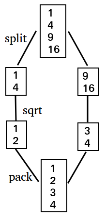
When performing a SQL query, MonetDB can speed up the query by splitting up the columns and running the query in parallel on multiple threads when possible. This is a process called mitosis. For example, when we want to take the square root of every element of a column, we can split up the column and have separate threads work on separate parts of the column. This is shown in the image below for a column of size 4 being split into two parts, and having two threads execute the operation.
However, certain operations cannot be parallelized because they require access to the entire column. These are called blocking operations. An example of such a blocking operation is the quantile function, because we cannot compute the quantile of a column when we only have access to part of a column. By default, embedded python is a blocking operation. This is because it is very easy to write a user defined function that is not mappable. We could, for example, use our python function to compute a quantile.
However, blocking operations are inefficient. When we use a blocking operation, we need to wait for all the previous threads to finish their operations. Then, we need to take all the split-up columns and recombine them into one big column, and then we can finally call the blocking operation. If our python function is mappable, we would prefer it to be executed in parallel.
Well, good news! We support this. If you know that your function is mappable, you can specify this by setting the LANGUAGE to PYTHON_MAP instead of PYTHON when creating the SQL function. Your function is mappable if the output does not depend on the entire column, but only on the individual rows.
For a simple example, let’s go back to the first function we created: multiplying a column of integers by 2. This is a mappable function, as the output works with the individual rows. The new function looks like this.
CREATE FUNCTION python_times_two_map (i INTEGER) RETURNS INTEGER
LANGUAGE PYTHON_MAP
{
    return i * 2
};
We can then use it just as we used the regular python_times_two function, and it will return the same result.
SELECT python_times_two_map(i) AS result FROM integers;
| result |
|---|
| 2 |
| 4 |
| 6 |
| 8 |
| 10 |
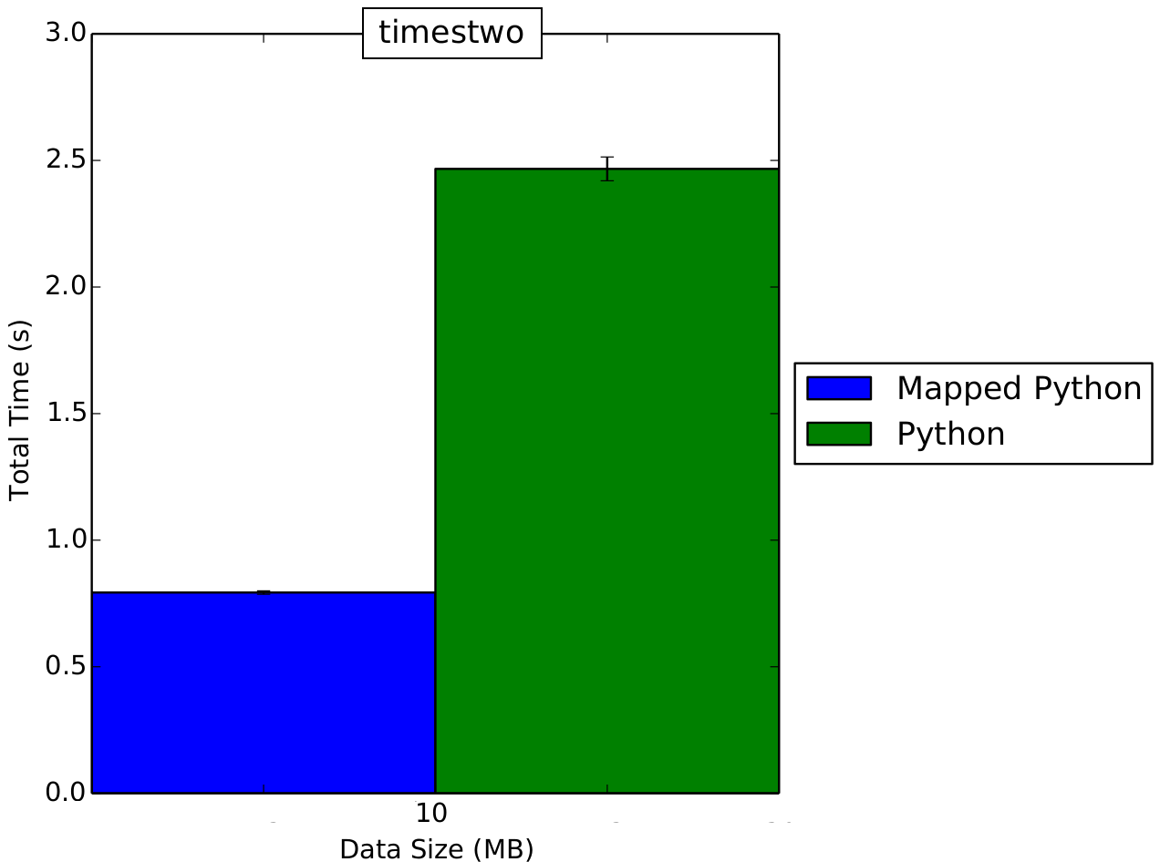
Even for such a simple function we can see a big performance increase when we increase the input size. Below is a graph running both functions with 1GB of input data.
Note that it is possible to run non-mappable functions using LANGUAGE PYTHON_MAP, however, this will then naturally produce different output than running the same function with LANGUAGE PYTHON. It is possible to abuse this to run part of a Python function in parallel. As an example, let’s make the MIN() function in our embedded Python.
Suppose we have the following mapped function, and the following non-mapped function.
CREATE FUNCTION python_min (i INTEGER) RETURNS integer
LANGUAGE PYTHON
{
    return numpy.min(i)
};

CREATE FUNCTION python_min_map (i INTEGER) RETURNS integer
LANGUAGE PYTHON_MAP
{
    return numpy.min(i)
};
At a glance these functions look identical. If we run the following query we will get the expected result.
SELECT python_min(i) FROM integers;
| min |
|---|
| 1 |
But if we run the mapped query we will get a different result [2].
SELECT python_min_map(i) FROM integers;
| min |
|---|
| 1 |
| 3 |
Since we are running with two threads, the function python_min_map is being executed twice. Once for one part of the column, and once for another part of the column. This means that the function returns two separate values. We can obtain the actual minimum value by using our sequential function python_min on the result of python_min_map.
SELECT python_min(python_min_map(i)) FROM integers;
| min |
|---|
| 1 |
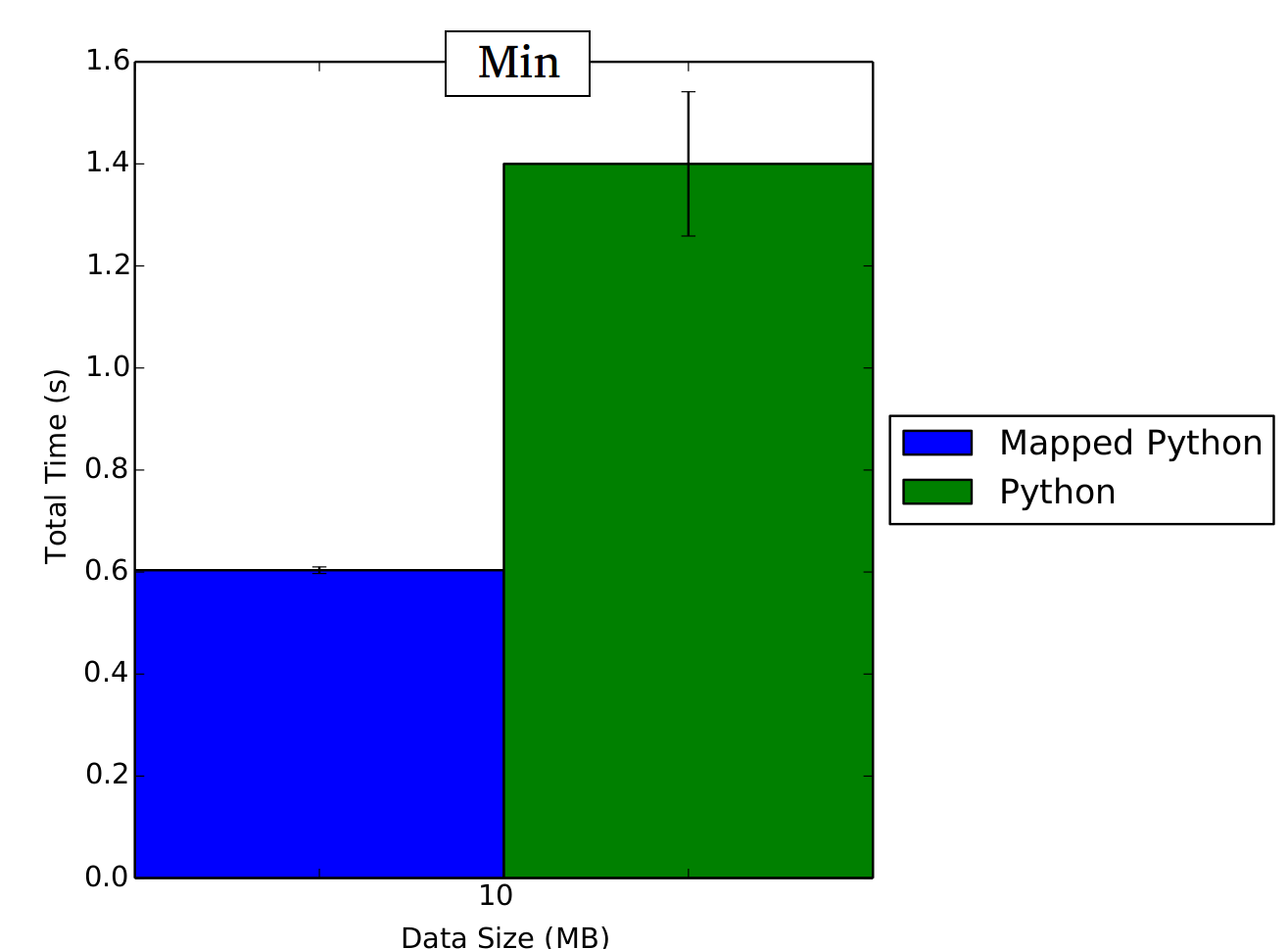
Now part of our query is being run in parallel, and we are still obtaining the desired result. Running these functions for a data set of 1000MB we can see that our parallel function has better performance than simply calling python_min, while still computing the correct value.
Performance
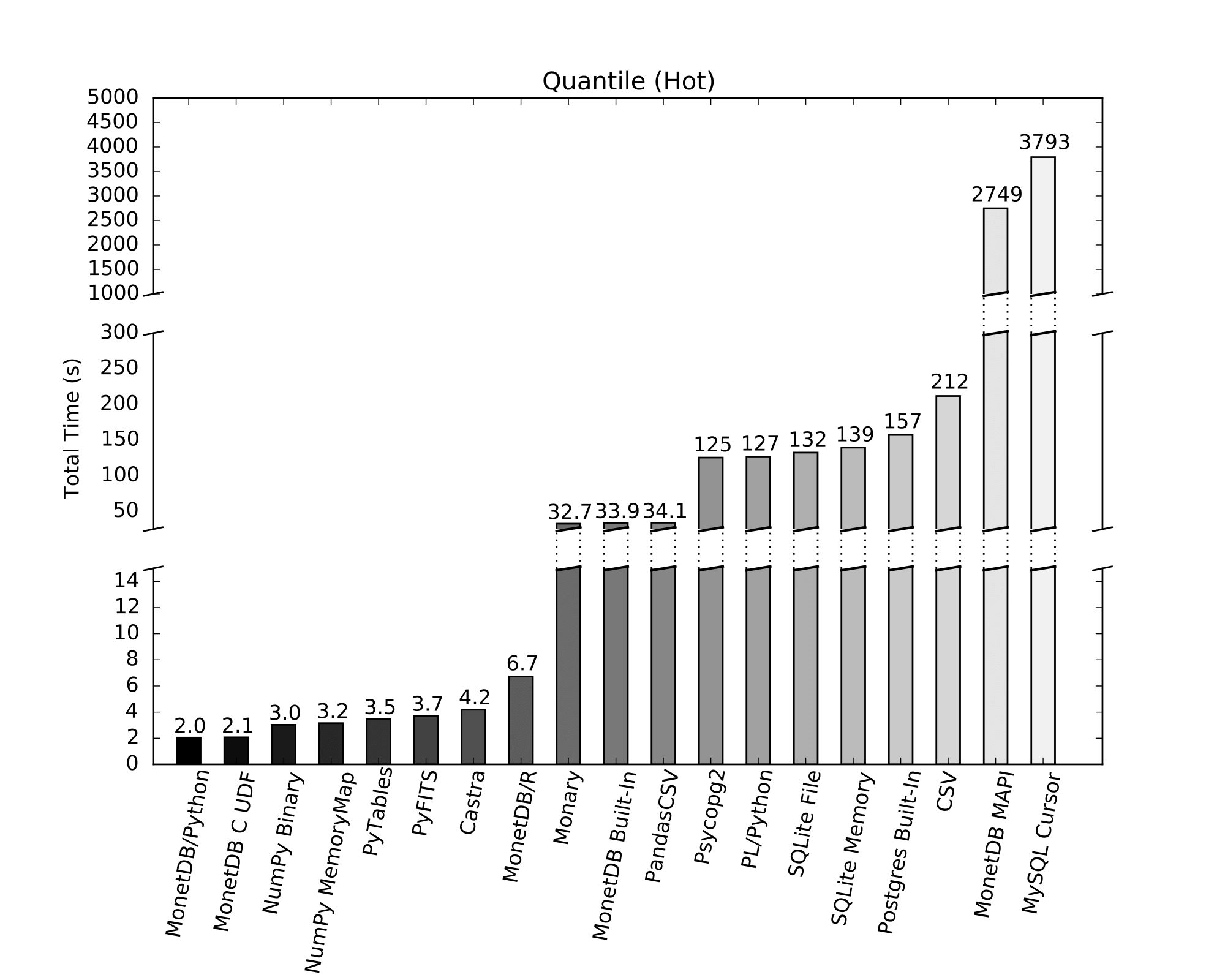
To keep in with tradition, we will use embedded python to compute quantiles. We can do this efficiently using the numpy.percentile function. We will compare our embedded Python implementation against various other ways of loading data into Python and then executing the numpy.percentile function on the data, as well as some other non-Python ways of computing the quantile. In our example, we are using a single table containing 1 GB of integer values (250M values).
- MonetDB/Python: This is our implementation, using numpy.percentile on the data within a MonetDB table. MonetDB uses memory mapping to load the data into memory very quickly, and because of our zero-copy transfer into Python there is no additional overhead cost for transferring this data into Python.
- MonetDB C UDF: Compute the quantile in MonetDB using a C UDF. We computed the quantile using Quickselect.
- NumPy Binary: Use numpy.load() to load the data into a numpy array from a numpy binary file. This is a very fast way of loading data into Python, because we are directly mapping a binary file into memory we do not have to do any decoding.
- NumPy MemoryMap: Use numpy.memmap() to load the data into a numpy array from a numpy binary file. This has similar performance to NumPy binary files.
- PyTables: Load the data using tables.open_file(). This is fast because it loads a binary file directly into a Numpy array.
- PyFITS: Use pyfits.open() to load the data from into a numpy array from a .fits file.
- castra: A column-store database created entirely in Python. This uses Python pickling to load the database file as a Python object from an encoded string. This has some additional overhead.
- MonetDB/R: Using the MonetDB/R library using the native R quantile function instead of the numpy.percentile function. The MonetDB/R extension does not use zero-copy transferring, which means there is extra overhead of copying the data once. In addition, it seems the numpy.percentile() function is faster than the quantile() function in R.
- Monary: Monary is a connector for MongoDB that is optimized for use with NumPy
- MonetDB Built-In: Use the built-in SQL quantile() function in MonetDB. This function does not use a very efficient algorithm for computing the quantile, which is why it takes a while.
- PandasCSV: Use the read_csv() function from the pandas library to load the data. This is an efficient C implementation of a CSV loader. However, we still need to decode the CSV and convert it into integer values, which means the loading takes a while.
- Psycopg2: Load the data into Python using psycopg2, the default Python connector for Postgres, and then use numpy.percentile() to compute the quantile. This is slow because it constructs individual Python objects for every integer.
- PL/Python: Load the data from a Postgres table using plpy.cursor() in a PL/Python function. This is slow because it loads the data as Python objects. There is also additional overhead from Postgres having to first gather all the relevant integer into a single array, as it is a row store database.
- SQLite: Call ‘SELECT * FROM table’ to load the data from SQLite into Python, using the built-in sqlite3 module. This implementation uses Python objects for integers instead of Numpy arrays, which carry a lot of additional overhead with regards to loading as we have to construct 250 million Python integer objects (which each have to be malloc’d individually).
- Postgres Built-In: Perform the quantile computation using the built-in percentile_cont aggregate, with Postgres tuned for Data Warehousing using pgtune.
- CSV: Use the built-in Python csv library to load the data into a Numpy array. This is much less efficient than the pandas load_csv() library as it constructs Python objects. In addition, the CSV loader is written in pure Python which carries additional overhead.
- MonetDB MAPI: Use the current MonetDB Python client to load the data into Python. This is extremely slow because data has to be serialized over sockets.
- MySQL Cursor: Load the data into Python using the MySQL Python Connector. This is extremely slow because it sends the data to Python one row at a time.
Discussion
We have shown that our embedded Python implementation is fast, however, the true strength of using Python is the fact that it is so flexible. All the functions we have shown here can easily be implemented in SQL as well.
In the next blog post we demonstrate that MonetDB/Python can be used for much more than just emulating simple SQL functions by performing classification, including preprocessing, training and predicting, of a big dataset using MonetDB/Python combined with SQL, without the data ever leaving MonetDB. This blog post can be found here.
We would like to make this integration generally available with the next feature release of MonetDB, till then we really would appreciate feedback at M.Raasveldt@cwi.nl .
Installation
Currently MonetDB/Python is available in the in-development version of MonetDB in the default branch and must be compiled from source. Note that you will need NumPy installed for embedded python to work. You can look here for information on how to install NumPy. To compile the pythonudf branch from scratch, you can download a tar file of the source here. You can then compile the source by running the following commands in the root directory of the source tree.
./bootstrap
./configure --prefix=<install_directory>
make
make install
You can then run MonetDB by starting the monetdbd daemon or mserver5 in the given installation directory. Note that you will need to explicitly enable Python integration using the following commands if you are using the monetdbd daemon.
monetdb stop pytest
monetdb set embedpy=true pytest
monetdb start pytest
Or the following command if you are running mserver5.
mserver5 --set embedded_py=true
You can then connect to MonetDB and use embedded python.
About the Author
Mark Raasveldt is studying Computer Science at Utrecht University. He is currently working on his Master’s thesis at the CWI Database Architectures Group. Surprisingly, he is working on embedding Python in MonetDB.
Footnotes
[1] The Numpy array is filled with Python objects of either type ‘str’ (if there are no unicode characters in the column) or ‘unicode’ (if there are unicode characters in the column).
[2] Note that we are running with 2 threads and forcing mitosis (mserver5 flags --set gdk_nr_threads=2 --forcemito), where --forcemito forces mitosis on small tables, otherwise MonetDB would not split up a table of 5 entries.


